Heat Demand Forecasting
Hylife Innovations
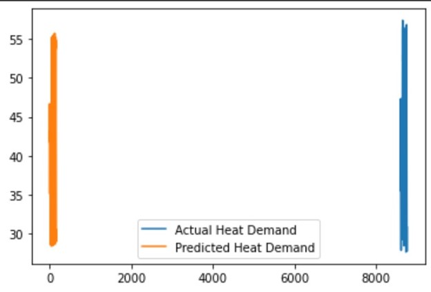
This project outlines the development of a heat demand forecasting algorithm designed to predict the hourly heat demand of the "HYLIFE OFFICE" building for the upcoming week. Developed in Python 3.9, the algorithm processes input data from an Excel file, which includes three normalized heat demand hourly profiles of generic buildings for 2021, related outside temperatures (in 0.1 °C), actual heat demand in kWh for HYLIFE OFFICE from the past year and January 2022, and forecasted outside temperatures for the period 1/2/2022 - 7/2/2022. The output is a heat demand forecast graph that is analyzed alongside historical data to assess accuracy and effectiveness. Several approaches were attempted to predict the heat demand of the Hylife offfice building such as simple linear regression, Vector Autoregression (VAR) model, and Long Short-Term Memory (LSTM) model to predict the heat demand.
Methodology
Linear Regression Model
First, a simple linear regression model was developed, but it was found to be inaccurate in predicting the heat demand due to the complex nature of the data. This model is a type of statistical model that seeks to establish a linear relationship between two variables, with one variable being the independent or predictor variable and the other variable being the dependent or response variable.

Vector Autoregression Model (VAR)
VAR is a statistical approach that models the relationships between multiple time series variables. It assumes that the variables in the system are influenced by their past values as well as the past values of other variables in the system. VAR is a good choice when the relationships between variables are relatively linear and stationary, and when there are not too many variables to model. It can also be useful when there are missing data points in the time series.
The code written is used to build a Vector AutoRegression (VAR) model to forecast the heat demand and energy consumption for a building.
Step 1 : The code begins by importing necessary libraries, such as statsmodels, pandas, numpy, and matplotlib. It also mounts the Google Drive to fetch the input data in the CSV format.
Step 2: This is followed by data preprocessing which includes converting the missing values to NaN and dropping them. The dataset is then plotted for visual inspection.
Step 3: The stationarity of each variable is tested using the Augmented Dickey-Fuller (ADF) test, and the Granger causality test is used to determine whether there is a causal relationship between two variables.
Step 4 : Next, the code prepares the data for modeling by splitting it into train and test datasets. The model used is VARMAX, which is a variant of the VAR model that includes exogenous variables. The order of the VAR model is determined using the select_order method, which determines the optimal lag length by evaluating different lag lengths and selecting the one with the lowest information criteria
Step 5 : Finally, the VARMAX model is fitted on the training dataset, and predictions are made on the test dataset. The predicted values are saved in the predictions variable, which can be used for further analysis and evaluation of the model's performance.

Long Short-Term Memory Model (LSTM)
Finally, a Long Short-Term Memory (LSTM) model was developed, which is a type of recurrent neural network that can model nonlinear relationships between variables and handle time series with complex patterns. It can capture long-term dependencies between the variables and adapt to changes in the data over time. LSTM is a good choice when there are many variables to model, or when the relationships between variables are highly nonlinear.
Step 1 : The code loads a CSV file containing the time series data and pre-processes it. It normalizes the data using StandardScaler, removes any NaN values, and saves the normalized data to a new CSV file. The preprocessed data is then used to train the LSTM model.
Step 2: The model is defined using the Sequential API from Keras. It consists of two LSTM layers with 64 and 32 units, respectively, followed by a Dropout layer with a rate of 0.2, and a Dense layer with one output unit. The model is compiled with the Adam optimizer and mean squared error (MSE) loss.
Step 3: The training data is divided into input sequences of length n_past and output sequences of length n_future, where n_past is the number of past time steps used to predict the next value and n_future is the number of future time steps to predict. The model is trained for a specified number of epochs and a batch size, and the training progress is saved to a history object.
Step 4 : Finally, the model is used to predict the next n_days_for_prediction values of the target feature, starting from the last n_past values in the training data. The predicted values are stored in a numpy array called prediction.

Analysis
In time series forecasting, accuracy may not be the best metric to evaluate the model's performance because it is a continuous output problem rather than a classification problem. Instead, using metrics such as Mean Squared Error (MSE), Root Mean Squared Error (RMSE), Mean Absolute Error (MAE), or Mean Absolute Percentage Error (MAPE) to evaluate the model's performance on the test set of the LSTM/ VAR model in time series forecasting.
RMSE (Root Mean Square Error) measures the average difference between the predicted and actual values. It is calculated by taking the square root of the mean of the squared differences between the predicted and actual values.
MAE (Mean Absolute Error) measures the average absolute difference between the predicted and actual values. It is calculated by taking the mean of the absolute differences between the predicted and actual values.
R-squared (R2) is a statistical measure that represents the proportion of variance in the dependent variable that is explained by the independent variables in the model. It ranges from 0 to 1, with higher values indicating better fit.
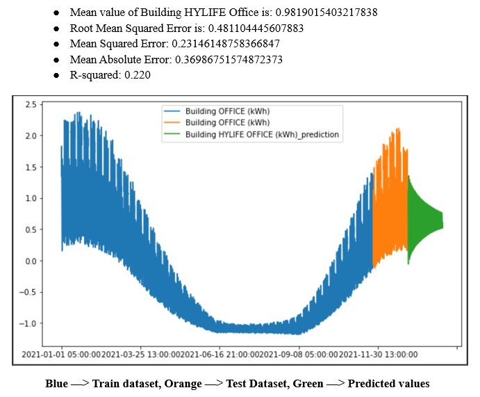
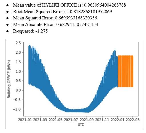
Based on these evaluation metrics, we can compare the performance of LSTM and VAR models trained on the same dataset as follows:

Conclusion
Based on the above results, it was concluded that the VAR model was a better choice in this particular case because it had a lower RMSE, MSE, and MAE values compared to the LSTM model. The R-squared value of the VAR model was also higher than the LSTM model, indicating that it was a better fit for the data.
VAR is generally considered a better approach than LSTM. Here are a few reasons why:
Possible Alternatives and Suggestions for improvements
Other models that can be used for time series forecasting include Prophet, ARIMA, and SARIMA. LSTM and VAR were chosen over this because they cannot handle multivariate data. It might further affect the accuracy of the model.
To improve the accuracy of the model, we can consider adding more variables such as humidity, wind speed, and solar radiation. We can also include a large dataset to predict a good model.